Native Gates

The IonQ Quantum Cloud has one of the best—-maybe the best—-optimizing compilers in quantum computing. This allows users to focus on the details of their algorithms instead of the details of our quantum system. You can submit quantum circuits using a large, diverse set of quantum gates that allows for maximum flexibility in how to define your problem, and our compilation and optimization stack ensures that your circuit runs on our QPUs in the most compact, streamlined, hardware-optimized form possible.

This flexibility in circuit definition also allows for high portability of algorithm code. We don’t restrict you to hardware-native basis gates, so you’re free to define in any gateset you want—-even the basis gates of a different hardware provider—-and then simply submit to IonQ hardware as-is. No changes necessary!

While this is ideal for many applications, the hardware-native basis gateset allows for more customizability, flexibility, and what-you-submit-is-what-you-get control. Being as “close to the metal” as possible allows for control over each individual gate and qubit, unlocking avenues of exploration that are impossible with a compiler between you and the qubits. Currently, submitting circuits defined in native gates is the only way to bypass the compiler and optimizer.

Read on to get started with our hardware-native gate specification, learn how it works, and run an example circuit using this powerful new ability.

​

When to use native gates

Native gates are not the right solution for every problem. As the warning above states, the native gate specification is an advanced-level feature. If your goal is simply to run a quantum circuit for evaluation or algorithm investigation purposes, using native gates will often result in lower-quality output than simply using the abstract gate interface.

The native gate interface is the simplest, most direct way to run a circuit on IonQ hardware: we run exactly the gates you submitted, as submitted, and we return the results. That’s it.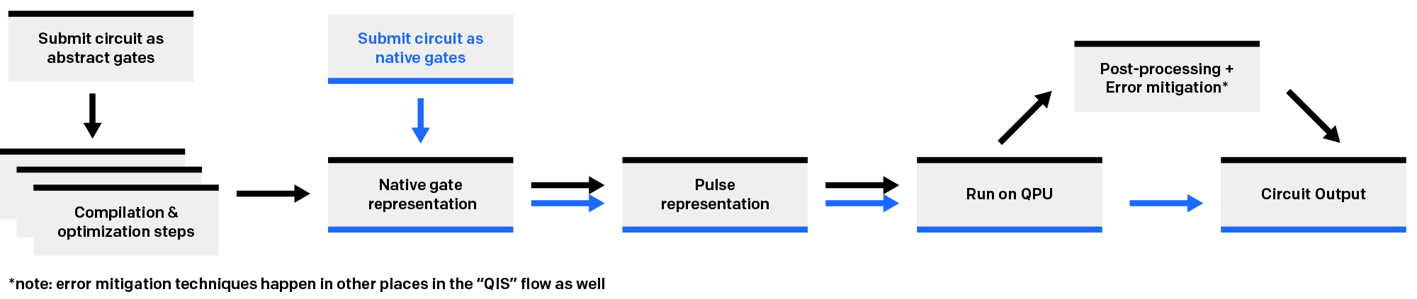

This means that our proprietary compilation and optimization toolchain is fully turned off when we execute a “native” circuit. (Error mitigation is also turned off by default, though you can choose to override this setting and turn on debiasing.) To take full advantage of our compilation, optimization, and error mitigation, you must submit your circuit using our default abstract gate interface, and if you are looking for maximum algorithmic performance from our systems, it is likely that you’ll find it by doing just that.

But, this toolchain performs a number of transformations on submitted circuits that we consider proprietary, and we therefore do not disclose the full details of how it works. By the time a circuit you submit through the abstract gate interface actually runs on hardware, it has been changed, sometimes considerably. Extraneous gates are optimized away or commuted into different places, they are transpiled into native gates using special heuristics and optimized again, and so on.

So, we recommend only using native gates when you cannot use the abstract interface to accomplish your goals - when you need to know exactly what circuit was run, or when you specifically want to run circuits that are not optimized. This might involve investigation and characterization of noise, designing noise-aware circuits, or exploring new error mitigation techniques, as well as the development and testing of circuit optimization and compilation methods.

​

Introducing the native gates

The native gateset is the set of quantum gates that are physically executed on IonQ hardware by addressing ions with resonant lasers via stimulated Raman transitions.

We currently expose two single-qubit gates and one two-qubit entangling gate for each QPU. Other native gates may be provided in the future.

All gate parameters are measured in turns rather than in radians: a value of 1 turn corresponds to 2π radians. We track the phase at the pulse level as units of turns—or, more accurately, as units of how long a turn takes—so, we expose the controls in the same way to you. This reduces floating point conversion error between what you submit and what runs.

​

Single-qubit gates

The “textbook” way to think about single-qubit gates is as rotations along different axes on the Bloch sphere, but another way to think about them is as rotations along a fixed axis while rotating the Bloch sphere itself.

Because, in physical reality, the Bloch sphere itself is rotating—that is, the phase is advancing in time—changing the orientation of the Bloch sphere is virtually noiseless on hardware. As such, we manipulate qubit states in this “noiseless” phase space whenever possible.

​

GPi

The GPi gate can be considered a π or bit-flip rotation with an embedded phase. It always rotates π radians—hence the name—but can rotate on any longitudinal axis of the Bloch sphere. At a ϕ of 0 turns this is equivalent to an X gate, and at a ϕ of 0.25 turns (π/2 radians) it is equivalent to a Y gate, but it can also be mapped to any other azimuthal angle.

$GPI(\phi) = \begin{bmatrix} 0 & e^{-i\phi} \\ e^{i\phi} & 0 \end{bmatrix}$

A single-qubit gate is physically implemented as a Rabi oscillation made with a two-photon Raman transition, i.e. driving the qubits on resonance using a pair of lasers in a Raman configuration. For more details on the physical gate implementation, we recommend this paper from the IonQ staff.

​

GPi2

The GPi2 gate could be considered an RX(π/2)—or RY(π/2)—rotation with an embedded phase. It always rotates π/2 radians but can rotate on any longitudinal axis of the Bloch sphere. At a ϕ of 0.5 turns (π radians) this is equivalent to RX(π/2), at a ϕ of 0.25 turns (π/2 radians) it is equivalent to RY(π/2), but it can also be mapped to any other azimuthal angle.

$GPI2(\phi)= \frac{1}{\sqrt{2}} \begin{bmatrix} 1 & -ie^{-i\phi} \\ -ie^{i\phi} & 1 \end{bmatrix}$

Like the GPi gate, the GPi2 gate is physically implemented as a Rabi oscillation made with a two-photon Raman transition.

​

Virtual Z

We do not expose or implement a “true” Z gate (sometimes also called a P or Phase Gate), where we wait for the phase to advance in time, but a Virtual RZ can be performed by simply advancing or retarding the phase of the following operation in the circuit. This does not physically change the internal state of the trapped ion at the time of its implementation; it adjusts the phases of the future operations such that it is equivalent to an actual Z-rotation around the Bloch sphere. In effect, virtual RZ operations are implied by the phase inputs to later gates.

$Virtual Z(\theta)= \begin{bmatrix} e^{-i\theta/2} & 0 \\ 0 & e^{i\theta/2} \end{bmatrix}$

For example, to add RZ(θ)—an RZ with an arbitrary rotation θ—to a qubit where the subsequent operation is GPi(0.5), we can just add that rotation to the phases of the following gates:

—RZ(θ)—GPI(0.5)—GPI2(0) = —GPI(θ + 0.5)—GPI2(θ + 0)

​

Entangling gates

For entangling gates, we offer different options for each QPU: the Mølmer-Sørenson gate on Aria-class systems, and the ZZ gate on our Forte-class systems.

​

MS gates

Invented in 1999 by several groups simultaneously, the Mølmer-Sørenson gate along with single-qubit gates constitutes a universal gate set. By irradiating any two ions in the chain with a predesigned set of pulses, we can couple the ions’ internal states with the chain’s normal modes of motion to create entanglement.

While it is possible to entangle many qubits simultaneously with the Mølmer-Sørenson interaction via global MS, or GMS, we only offer two-qubit MS gates at this time.

Fully entangling MS

The fully entangling MS gate is an XX gate—a simultaneous, entangling π/2 rotation on both qubits. Like our single-qubit gates, they nominally follow the X axis as they occur, but take two phase parameters that make e.g. YY or XY also possible. The first phase parameter ϕ₀ refers to the first qubit’s phase (measured in turns) as it acts on the second one, the second parameter ϕ₁ refers to the second qubit’s phase (measured in turns) as it acts on the first one.

If both are set to zero, there is no advancing phase between the two qubits because the transition is driven on both qubits simultaneously, in-phase. That is, the relative phase between the two qubits remains the same during the operation unless a phase offset is provided.

$MS(\phi_0, \phi_1) = \frac{1}{\sqrt{2}} \begin{bmatrix} 1 & 0 & 0 & -ie^{-i(\phi_0 + \phi_1)} \\ 0 & 1 & -ie^{-i(\phi_0 - \phi_1)} & 0 \\ 0 & -ie^{i(\phi_0 - \phi_1)} & 1 & 0 \\ -ie^{i(\phi_0 + \phi_1)} & 0 & 0 & 1 \end{bmatrix}$

Note that while two distinct ϕ parameters are provided here (one for each qubit, effectively), they always act on the unitary together. This means that there are multiple ways to get to the same relative phase relationship between the two qubits for this gate; two parameters just makes the recommended approach of “Virtual Z” phase accounting on each qubit across the entire circuit a little neater.

Partially entangling MS

In addition to the fully entangling MS gate described above, we also support partially entangling MS gates, which are useful in some cases. To implement these gates, we add a third (optional) arbitrary angle θ:

$\text{MS}(\phi_0,\phi_1,\theta) = \begin{bmatrix} \cos \frac{\theta}{2} & 0 & 0 & -i e^{-i(\phi_0+\phi_1)} \sin \frac{\theta}{2} \\ 0 & \cos \frac{\theta}{2} & -i e^{-i(\phi_0-\phi_1)} \sin \frac{\theta}{2} & 0 \\ 0 & -i e^{i(\phi_0-\phi_1)} \sin \frac{\theta}{2} & \cos \frac{\theta}{2} & 0 \\ -i e^{i(\phi_0+\phi_1)} \sin \frac{\theta}{2} & 0 & 0 & \cos \frac{\theta}{2} \end{bmatrix}$

This parameter is also measured in turns, and can be any floating-point value between 0 (identity) and 0.25 (fully-entangling); in practice, the physical hardware is limited to around three decimal places of precision. Requesting an MS gate without this parameter will always run the fully entangling version.

Partially entangling MS gates yield more compact circuits: to produce the same effect as one arbitrary-angle MS gate would require up to two fully-entangling MS gates plus four single-qubit rotations. This offers a potential reduction in gate depth that can indirectly improve performance by removing unnecessary gates in certain circuits.

Additionally, small-angle MS gates are generally more performant: for smaller angles, these gates are implemented by lower-power laser pulses, and therefore experience lower light shift and other power-dependent errors. We do not currently have a detailed characterization of how much more performant these gates are on our current-generation systems, but in our (now-decommissioned) system described in this paper, we saw an improvement from ~97.5% to ~99.6% two qubit fidelity when comparing angles of π/2 and π/100, which is described in more detail here.

​

ZZ gates

Our Forte systems use the ZZ gate, which is another option for creating entanglement between two qubits. Unlike the Mølmer-Sørenson gate, the ZZ gate only requires a single parameter, θ, to set the phase of the entanglement.

$ZZ(\theta) = \exp\left(-i \frac{\theta}{2} Z{\otimes}Z\right) = \begin{pmatrix} e^{-i \frac{\theta}{2}} & 0 & 0 & 0 \\ 0 & e^{i \frac{\theta}{2}} & 0 & 0 \\ 0 & 0 & e^{i \frac{\theta}{2}} & 0 \\ 0 & 0 & 0 & e^{-i \frac{\theta}{2}} \end{pmatrix}$

​

Converting to native gates

You can write a quantum circuit using native gates directly, but you can also convert an abstract-gate circuit into native gates. To do this automatically, we support Qiskit’s transpiler. Here, we’ll walk through the general approach for manually translating circuits into native gates.

​

General algorithm

To translate anything into native gates, the following general approach works well:

1. Decompose the gates used in the circuit so that each gate involves at most two qubits.

2. Convert all easy-to-convert gates into RX, RY, RZ, and CNOT gates.

3. Convert CNOT gates into XX gates using the decomposition described here and at the bottom of this section.

4. For hard-to-convert gates, first calculate the matrix representation of the unitary, then use either KAK decomposition or the method introduced in this paper to implement the unitary using RX, RY, RZ and XX. Note that Cirq and Qiskit also have subroutines that can do this automatically, although potentially not optimally. See cirq.linag.kak_decomposition and qiskit.synthesis.TwoQubitBasisDecomposer.

5. Write RX, RY, RZ and XX into GPi, GPi2 and MS gates as documented above (making sure to convert all angles and phases from radians to turns).

​

CNOT to XX decomposition

A CNOT gate can be expressed in XX, RX, and RY gates which can be directly converted to IonQ’s native gates.

----@-----   ----| RY(π/2) |----|         |----| RX(-π/2) |----| RY(-π/2) |-----
    |      =                    | XX(π/4) |
----X-----   -------------------|         |----| RX(-π/2) |---------------------

Many more advanced approaches, decompositions, and optimizations for trapped-ion native gates, including a parameterizable version of this decomposition can be found in Basic circuit compilation techniques for an ion-trap quantum machine, where this decomposition is described.

​

Additional resources

To learn how to use native gates via the IonQ API and supported SDKs:

• Native gates in the IonQ API
• Native gates in Qiskit
• Native gates in Cirq
• Native gates in PennyLane

For those interested in learning more about trapped-ion quantum computers as a physical apparatus, the implementation of gates, etc, we recommend the PhD theses from our cofounder Chris Monroe’s lab as a starting point, especially those of Debnath, Egan, Figgat, Landsman, and Wright. The hardware they describe is in many ways the “first iteration” of IonQ’s hardware, and much of the fundamental physics of the trapped-ion approach carries over.