Hosted Hybrid Service

The Hosted Hybrid service is currently in a limited preview and only available to customers with an active contract. Please contact [email protected] for more information.

IonQ’s Hosted Hybrid Service allows users to run hybrid quantum-classical workloads without needing to write or host the classical optimization logic. This means that you can run a hybrid algorithm like a VQE, optimize the inputs with a method like SPSA, and do it all without having to write-or-run any of the code yourself. This service introduces a two new things to our platform: A Quantum Function is an abstraction that represents a composition of classical and quantum logic to perform simple computations. We currently expose two types of Quantum Functions:

Hamiltonian Energy, which takes an ansatz and a hamiltonian to perform hamiltonian energy evaluation.
Quadratically Constrained Quadratic Program that models the objective of a (constrained) quadratic program. This QuantumFunction can be used to solve constrained quadratic programs.

An Optimization looks for the optimal parameters for a Quantum Function using a supported optimization function. Once completed, the solution returned is the minimum energy value and the optimal parameters used to achieve it. These new tools allow you take a problem that you want to solve, represent it in the form of a function, and run it through an optimization routine—without having to run any of the classical code yourself in a local notebook, or manage a remote execution environment.

Setup

To run hybrid workloads with this tool, you’ll need:

Python 3.9 or greater

We recommend using a version manager such as pyenv or asdf to simplify management and upgrades.

The IonQ SDK and all its extras

pip install 'ionq[all]'

We’ll start by setting up our our Client which will allow us to connect to IonQ’s platform, then select a backend to use with it.

# Initialize backend
from ionq.client import Client
from ionq import Backend

# Initialize a client for connecting to the IonQ API
client = Client()

# Note: Assuming it's stored as $IONQ_API_KEY in your environment,
# the SDK (and any other quantum SDK) will find it automatically.
# However, if you wanted to specify it directly, you could with:
# client = Client(api_key="aaa-bbb-ccc")

# Select a backend to use. We'll stick with the simulator for now, but you can
backend = Backend(name="simulator", client=client)

Creating a demo workload

In practice, you’d be using our hamiltonian energy evaluations to evaluate your own hamiltonians and ansatze, but for this guide we’ll build a couple of functions for creating random inputs — but if you can provide your own, more the better. So first, we’ll build an example hamiltonian:

import random
import math
from itertools import product

from qiskit.quantum_info import SparsePauliOp

# Create our example hamiltonian

num_qubits = 2  # or more, but it scales rapidly!

pauli_list = [
    (ps, random.uniform(-1, 1))
    for ps in [
        "".join(p) for p in list(product(["I", "X", "Y", "Z"], repeat=num_qubits))
    ]
]

# Create and display an example hamiltonian
hamiltonian = SparsePauliOp.from_list(pauli_list)

Which, if we printed it, would look something like:

print(hamiltonian.to_matrix())

[[-0.66819263+0.j         -1.36722223-1.22394246j  1.61219673+1.45550222j
   0.1523982 -1.25363417j]
 [-1.36722223+1.22394246j  1.40731579+0.j         -1.42421166+0.51092863j
  -0.16465104-0.43298482j]
 [ 1.61219673-1.45550222j -1.42421166-0.51092863j  0.86269394+0.j
  -0.388201  -0.74335051j]
 [ 0.1523982 +1.25363417j -0.16465104+0.43298482j -0.388201  +0.74335051j
   2.28670504+0.j        ]]

Now we’ll do the same for an example ansatz and some initial parameters:

from qiskit import QuantumCircuit
from qiskit.circuit import Parameter

params = [Parameter(f"θ{i}") for i in range(2 * num_qubits)]
ansatz = QuantumCircuit(num_qubits)

# Add a layer of single-qubit parameterized rotations (Ry and Rz)
for i in range(num_qubits):
    ansatz.ry(params[i], i)
    ansatz.rz(params[i + num_qubits], i)

ansatz.barrier()

# Add CNOT gates to entangle the qubits
for i in range(num_qubits - 1):
    ansatz.cx(i, i + 1)

# Set up some initial parameters
initial_params = {
    params[i]: random.uniform(0, 2 * math.pi) for i in range(2 * num_qubits)
}

Which will produce an ansatz that looks something like:

ansatz.draw(output="mpl")

Example 1: Running a simple circuit

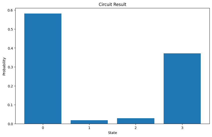
As a simple demonstration of functionality, let’s take our backend and submit a basic circuit job to it using our example ansatz. This is not a hybrid workflow, but a normal circuit job. Note: We’re using ionq.ionq_qiskit, which is a helper library we are providing for translating Qiskit circuits into IonQ-native QIS.

from ionq.utils import ionq_qiskit

# Create a circuit using a helper that translates Qiskit circuits to QIS
circuit = ionq_qiskit.to_circuit(
    [ansatz.assign_parameters(initial_params, inplace=False)]
)

# And submit it to our backend
circuit_job = backend.run(
    circuit,
    name="Example 1: Circuit Workload"
)

And plotting this circuit we’ll see something like:

circuit_results = circuit_job.results()
for results in circuit_results:
    results.plot_results()

Example 2: Running a Quantum Function

Now we’re build on this by submitting a QuantumFunction instead of just a simple circuit. A quantum function is a workload that has some predefined logic built in to it. In this case, we’ll pass it an ansatz and a hamiltonian, and when we send it to the backend along with a set of parameters, it will submit circuits and do an Hamiltonian Energy evaluation.

from ionq.jobs import HamiltonianEnergy
from ionq.utils import ionq_qiskit

# Build a QuantumFunction
qfunc = HamiltonianEnergy(
    ansatz=ionq_qiskit.to_ansatz(ansatz),
    hamiltonian=ionq_qiskit.to_hamiltonian(hamiltonian),
)

# Submit it to the backend
qfunc_job = backend.run(
    qfunc,
    params=list(initial_params.values()),
    name="Example 2: Quantum Function Workload",
)

Example 3: Quadratically Constrained Quadratic Program Objective

We can also prepare the model for a constrained quadratic program, by creating a Quantum Function that takes an ansatz, a QUBO matrix, and a list of constraints. This can then be used to solve constrained quadratic programs with classical optimization methods. Let’s first model it, with some simple linear constraints and confirm it runs with a random set of parameters.

import numpy as np

from ionq.problems.quadratic import LinearConstraint
from ionq.problems import QCQPObjective
from ionq.utils import ionq_qiskit

Q = np.array([[4, -6], [-6, 10]])

constraints = [
    LinearConstraint(
        coeffs=[1, 2],
        rhs=5,
     ),
    LinearConstraint(
        coeffs=[3, 4],
        rhs=6,
    )
]

print(f"{Q=}", "\n\n", f"{constraints=}")

# Build our QuantumFunction
qfunc = QCQPObjective(
    ansatz=ionq_qiskit.to_ansatz(ansatz),
    qp_objective=Q,
    linear_constraints=constraints,
    penalty=random.uniform(-1, 1),
)

# Submit it to the backend
qfunc_job = backend.run(
    qfunc,
    params=list(initial_params.values()),
    name="Example 3: Quantum Function (with constraints and a penalty)",
)

Example 4: Optimizations

We can also run a (IonQ hosted!) classical loop to optimize our parameters. Here we’ll take the same quantum function we ran in Example 3, but we’ll add a 5-iteration optimization using SPSA. It doesn’t add that much complexity here, only requiring some simple additions:

What method to use for optimization
The maximum desired number of iterations
The learning rate, and perturbation for each iteration

These values will define how each iteration in the series will change based on the results of the previous job.

from ionq.jobs import Optimization
from ionq.jobs import OptimizationMethod

opt = Optimization(
    quantum_function=qfunc,
    method=OptimizationMethod.SPSA,
    initial_params=list(initial_params.values()),
    log_interval=1,
    options={"maxiter": 5, "learning_rate": 0.1, "perturbation": 0.5},
    maxiter=5,
)

# Run the optimization job
opt_job = backend.run(
    opt,
    name="Example 4: Optimization"
)

As before, we’ve provided some useful helpers for visualization. running plot_results() gives us:

opt_results = opt_job.results()
opt_results.plot_results()

A graph of the results of an optimization job.

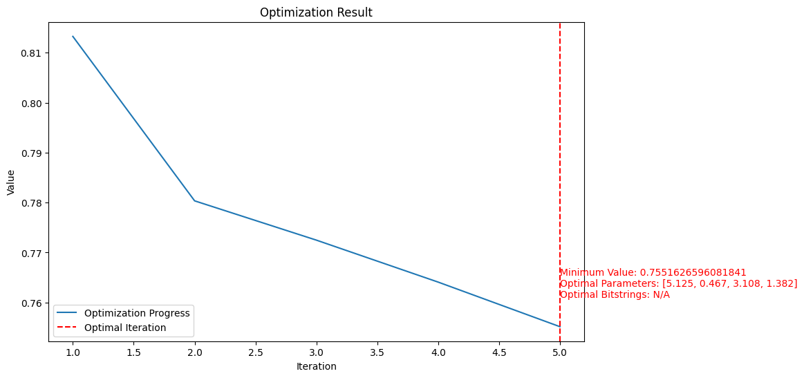
And retrieving the “results” of this job will identify the minimum_value and optimal_parameters for the problem:

"solution": {
    "minimum_value": -0.6128005853629444,
    "optimal_parameters": [
        4.915170460439439,
        3.228145593574783,
        5.550801246532398,
        -0.012326729967622713
    ]
}

Learn more

This service is still in a private alpha at this time, but reach out to [email protected] for more information, or contact your account manager.

Introduction

Features

Guides

User Manual

Access Partners

Integrations

Setup

Creating a demo workload

Example 1: Running a simple circuit

Example 2: Running a Quantum Function

Example 3: Quadratically Constrained Quadratic Program Objective

Example 4: Optimizations

Learn more

​Setup

​Creating a demo workload

​Example 1: Running a simple circuit

​Example 2: Running a Quantum Function

​Example 3: Quadratically Constrained Quadratic Program Objective

​Example 4: Optimizations

​Learn more

Setup

Creating a demo workload

Example 1: Running a simple circuit

Example 2: Running a Quantum Function

Example 3: Quadratically Constrained Quadratic Program Objective

Example 4: Optimizations

Learn more